
Descriptive statistics and correlations are every data scientists’ bread and butter, but they often come with the caveat that correlation isn’t causation. At Shopify, we believe that understanding causality is the key to unlocking maximum business value. We aim to identify insights that actually indicate why we see things in the data, since causal insights can validate (or invalidate) entire business strategies. Below I’ll discuss different causal inference methods and how to use them to build great products.
The Causal Inference “Levels of Evidence Ladder”
A data scientist can use various different methods to estimate the causal effects of a factor. The “levels of evidence ladder” is a great mental model that introduces the ideas of causal inference.

Levels of evidence ladder. First level (clearest evidence): A/B tests (a.k.a statistical experiments). Second level (reasonable level of evidence): Quasi-experiments (including difference-in-differences, matching, controlled regression). Third level (weakest level of evidence): Full estimation of counterfactuals. Bottom of the chart: descriptive statistics—provides no direct evidence for causal relationship.
The ladder isn’t a ranking of methods, instead it’s a loose indication of the level of proof each method will give you. The higher the method is on the ladder, the easier it is to compute estimates that constitute evidence of a strong causal relationship. Methods at the top of the ladder typically (but not always) require more focus on the experimentation setup. On the other end, methods at the bottom of the ladder use more observational data, but require more focus on robustness checks (more on this later).
The ladder does a good job of explaining that there is no free lunch in causal inference. To get a powerful causal analysis you either need a good experimental setup, or a good statistician and a lot of work. It’s also simple to follow. I’ve recently started sharing this model with my non-data stakeholders. Using it to illustrate your work process is a great way to get buy-in from your collaborators and stakeholders.
Causal Inference Methods
A/B tests
A/B tests, or randomized controlled trials, are the gold standard method for causal inference—they’re on rung one of the levels of evidence ladder! For A/B tests, group A and group B are randomly assigned. The environment both groups are placed in is identical except for one parameter: the treatment. Randomness ensures that both groups are clones “on average”. This enables you to deduce causal estimates from A/B tests, because the only way they differ is the treatment. Of course in practice, lots of caveats apply! For example, one of the frequent gotchas of A/B testing is when the units in your treatment and control groups self-select to participate in your experiment.
Setting up an A/B test for products is a lot of work. If you’re starting from scratch, you’ll need
- A way to randomly assign units to the right group as they use your product.
- A tracking mechanism to collect the data for all relevant metrics.
- To analyze these metrics and their associated statistics to compute effect sizes and validate the causal effects you suspect.
And that only covers the basics! Sometimes you’ll need much more to be able to detect the right signals. At Shopify, we have the luxury of an experiments platform that does all the heavy work and allows data scientists to start experiments with just a few clicks.
Quasi-experiments
Sometimes it’s just not possible to set up an experiment. Here are a few reasons why A/B tests won’t work in every situation:
- Lack of tooling. For example, if your code can’t be modified in certain parts of the product.
- Lack of time to implement the experiment.
- Ethical concerns for example, at Shopify, randomly leaving some merchants out of a new feature that could help them with their business is sometimes not an option).
- Just plain oversight (for example, a request to study the data from a launch that happened in the past).
Fortunately, if you find yourself in one of the above situations, there are methods that exist which enable you to obtain causal estimates.
A quasi-experiment (rung two) is an experiment where your treatment and control group are divided by a natural process that isn’t truly random, but are considered close enough to compute estimates. Quasi-experiments frequently occur in product companies, for example, when a feature rollout happens at different dates in different countries, or if eligibility for a new feature is dependent on the behaviour of other features (like in the case of a deprecation). In order to compute causal estimates when the control group is divided using a non-random criterion, you’ll use different methods that correspond to different assumptions on how “close” you are to the random situation.
I’d like to highlight two of the methods we use at Shopify. The first is linear regression with fixed effects. In this method, the assumption is that we’ve collected data on all factors that divide individuals between treatment and control group. If that is true, then a simple linear regression on the metric of interest, controlling for these factors, gives a good estimate of the causal effect of being in the treatment group.
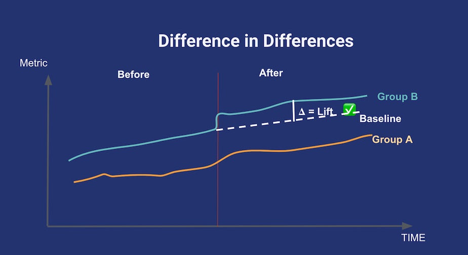
The parallel trends assumption for differences-in-differences. In the absence of treatment, the difference between the ‘treatment’ and ‘control’ group is a constant. Plotting both lines in a temporal graph like this can help check the validity of the assumption. Credits to Youcef Msaid.
The second is also a very popular method in causal inference: difference in difference. For this method to be applicable, you have to find a control group that shows a trend that’s parallel to your treatment group for the metric of interest, prior to any treatment being applied. Then, after treatment happens, you assume the break in the parallel trend is only due to the treatment itself. This is summed up in the above diagram.
Counterfactuals
Finally, there will be cases when you’ll want to try to detect causal factors from data that only consists of observations of the treatment. A classic example in tech is estimating the effect of a new feature that was released to all the user base at once: no A/B test was done and there’s absolutely no one that could be the control group. In this case, you can try making a counterfactual estimation (rung three).
The idea behind counterfactual estimation is to create a model that allows you to compute a counterfactual control group. In other words, you estimate what would happen had this feature not existed. It isn’t always simple to compute an estimate. However, if you have a model of your users that you’re confident about, then you have enough material to start doing counterfactual causal analyses!
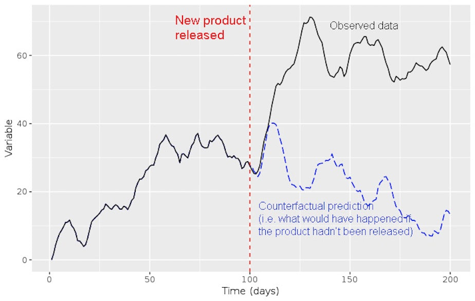
Example of time series counterfactual vs. observed data
A good way to explain counterfactuals is with an example. A few months ago, my team faced a situation where we needed to assess the impact of a security update. The security update was important and it was rolled out to everyone, however it introduced friction for users. We wanted to see if this added friction caused a decrease in usage. Of course, we had no way of finding a control group among our users.
With no control group, we created a time-series model to get a robust counterfactual estimation of usage of the updated feature. We trained the model on data such as usage of other features not impacted by the security update and global trends describing the overall level of activity on Shopify. All of these variables were independent from the security update we were studying. When we compared our model’s prediction to actuals, we found that there was no lift. This was a great null result which showed that the new security feature did not negatively affect usage.
When using counterfactual methods, the quality of your prediction is key. If a confounding factor that’s independent from your newest rollout varies, you don’t want to attribute this change to your feature. For example, if you have a model that predicts daily usage of a certain feature, and a competitor launches a similar feature right after yours, your model won’t be able to account for this new factor. Domain expertise and rigorous testing are the best tools to do counterfactual causal inference. Let’s dive into that a bit more.
The Importance of Robustness
While quasi-experiments and counterfactuals are great methods when you can’t perform a full randomization, these methods come at a cost! The tradeoff is that it’s much harder to compute sensible confidence intervals, and you’ll generally have to deal with a lot more uncertainty—false positives are frequent. The key to avoiding falling into traps is robustness checks.
Robustness really isn't that complicated. It just means clearly stating assumptions your methods and data rely on, and gradually relaxing each of them to see if your results still hold. It acts as an efficient coherence check if you realize your findings can dramatically change due to a single variable, especially if that variable is subject to noise, error measurement, etc.
Direct Acyclic Graphs (DAGs) are a great tool for checking robustness. They help you clearly spell out assumptions and hypotheses in the context of causal inference. Popularized by the famous computer scientist, Judea Pearl, DAGs have gained a lot of traction recently in tech and academic circles.
At Shopify, we’re really fond of DAGs. We often use Dagitty, a handy browser-based tool. In a nutshell, when you draw an assumed chain of causal events in Dagitty, it provides you with robustness checks on your data, like certain conditional correlations that should vanish. I recommend you explore the tool
The Three Most Important Points About Causal Inference
Let’s quickly recap the most important points regarding causal inference:
- A/B tests are awesome and should be a go to tool in every data science team’s toolbox.
- However, it’s not always possible to set up an A/B test. Instead, look for natural experiments to replace true experiments.
- If no natural experiment can be found, counterfactual methods can be useful. However, you shouldn’t expect to be able to detect very weak signals using these methods.
I love causal inference applications for business and I think there is a huge untapped potential in the industry. Just like generalizing A/B tests lead to building a very successful “Experimentation Culture” since the end of the 1990s, I hope the 2020s and beyond will be an era of the “Causal Culture” as a whole! I hope sharing how we do it at Shopify will help. If any of this sounds interesting to you, we’re looking for talented data scientists to join our team.